Ever wish you had your gridlines, column letters and row numbers on the printout of an MS Excel worksheet?

On some of the larger worksheets or on worksheets where there aren't a lot of labels on the data, this tip could be the little "miracle" you've been looking for. Okay, maybe the word miracle is a bit strong, daily cialis results but then again, it all depends on how lost you've become in your data. It's all in the perspective!

I know sometimes I just have to see it in print to find the mistakes. If only that would ensure I could catch them all. I don't know about you, but some days, my mistake list seems endless!

At any rate, once you've made the decision that you need your gridlines and/or headings, your solution is just a few clicks away.

For people using older versions of Excel, your solution is found in the Page Setup information. So, we'll begin by going to the File menu, Page Setup choice.

Once the Page Setup window opens, you're looking for the Sheet tab.

In the middle section, called Print, you're looking for the Gridlines and Row and Column Headings checkboxes.

Make sure you select the items you need.

Click OK.

For Excel 2007 users, you need the Page Layout ribbon.

Check the Print box for Headings and/or Gridlines as necessary.

There you have it. All the labels and gridlines you could ever want!

Now, you know where to find everything!

Here's a little tidbit that comes from a reader's question!

The reader was having difficulty with MS Excel's column labeling cialis wiki feature. Instead of letters for column headers, she had numbers.

(Did you notice the cell name given in the corner? Obviously not what most of you are used to).

It was driving her crazy, because it didn't match the other systems she worked on at school and/or work.

So, what's the deal here? Is the one system just "out of whack" or what?

Can it be "fixed?"

Good questions!

Yes, it can be fixed!

To retrieve your beloved letter headings, simply begin with Excel's Options.

For older versions of Excel, they're found via the Tools menu, Options choice.

In the Options dialogue window, you're looking for the General tab.

In Excel 2007, you need the Excel Options button, which is located in the bottom right corner of the Office Button menu.

You need the Formulas section under Excel's options.

In any version, you'll need to uncheck the "R1C1 reference style" box.

Click OK.

Poof!

Your missing letters have been returned. If only everything could be so easy to retrieve!

Have you ever had an MS Excel workbook that you're constantly working in, making the same changes to several different worksheets?

What did you do?

Did you go to the first sheet, make changes, move to the next sheet, make the same changes, move to the next sheet, make the same changes again and so on?

How tiresome was that?

Want a quicker way to make identical changes on different sheets?

Maybe a way that allows you to make just one set of changes that will include all of the necessary worksheets?

Sounds too good to be true, doesn't it?!

Well, there's no need to pinch yourself. You're not dreaming. It can be done and it doesn't require any special feature or function. You just have to know about a couple extra clicks!

Ready to get started?

Yes?

Good, let's get going!

• The first thing you need to do is go to the first worksheet to be changed/edited.

• Next, you need to select the sheet tabs of all the worksheets that need the same changes.

  • To select a series of tabs, hold down the Shift key and click on the last sheet tab in the series. You should see that the first, last and all tabs in between are selected simultaneously.

  • If you have non-consecutive sheets to change, hold down the Ctrl key and click on the tab for each sheet cialis wholesale to be changed.

• Once you have all the tabs selected, you're ready to begin your changes.

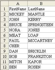
I'm sure you've all used cell references in your MS Excel formulas, right? You know, let's say you want to add cells A2 and A3 and write a formula to do this in another location. Maybe even something as simple as =A2 + A3.

These formulas are great and pretty easy to use, but let's say there's a piece of data from one worksheet that you need to bring to another. What do you do then?

If cialis trial pack there's a chance the number from the other worksheet could change, you don't want to simply copy the number into the new worksheet. A move like that would only cause you grief. Every time you make a change that altered the value, you'd have to remember to retype the new number on the second worksheet as well.

Forget it! That method isn't worth the trouble.

Let's face it, if you can't set your workbook up to run smoothly and keep updates you have to make to a minimum, you're just looking for some trouble. You'll inevitably overlook one of those repetitive updates and the data will be meaningless.

So, now what?

The solution I suggest is to use the cell locations from the other worksheets in the formula, just like you would if the cells were located all on the same sheet.

Okay, so it isn't exactly the same. There is a slight difference in the way you reference the cells, but once you understand the new references, it's smooth sailing from there.

Now that we know why we want to use references for cells from different worksheets, let's get busy with the how to!

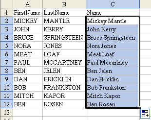
We all know about the basic formula to add two cells from within the same worksheet where the formula will be used. Let's use the one from above as our example: =A2 + A3

Now, let's just say that instead of A2 and A3 from the current worksheet, you want to use A2 from Sheet2 and A3 from Sheet3 in the workbook.

The new formula (with the different sheet references) would look like this: =Sheet2!A2+Sheet3!A3

Your formula has to somehow tell Excel where to find the cells in the workbook and do it before the cell location with the sheet name and the exclamation point. (Without the extra clarification, the program simply uses the sheet with the formula).

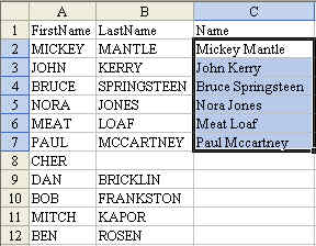
After using a formula like that, you're relieved from any extra updating! If you change a number in either of those cells, the formula will automatically update using the new values.

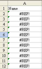
This type of referencing works in any formula, but you have to be sure not to have any typos in the sheet name. Excel will not guess what you mean, because it only works very literally.

What's that? You don't like all the extra typing? You're more of a "clicker" when it comes to building your formulas?

No problem!

You already know you can click to a cell location to insert it into a formula and well, it works the same way here.

• Start your formula with the equal sign.

• Use the sheet tabs (or Ctrl + Page Up/Page Down) to move to another worksheet in the workbook.

• Click on the cell(s) you need inserted into the formula.

• At this point, do not click back to the sheet you're working on, just simply continue inserting the elements (cell locations and keystrokes) of your formula.

• When you complete the formula, hit the Enter key.