|
I teach a class on Power Excel at the University of Akron. Although it is advertised as an advanced class, there are always some basic concepts that the students don't seem to know. I am amazed at how the simplest techniques will cause the most excitement. This is one of those tips.
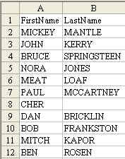
Today, Sajjad from Dubai wrote with a question. He has a database with first name in Column A and Last name in column B. How can he merge First Name and Last Name into a single column?
This is one of those questions that you can never find in Excel help, because no one thinks to search for the word "Concatenation". Heck, I don't think any normal person ever uses the word concatenate. If you don't know to search for Concatenate, then you will never learn that the concatenation operator is an ampersand. Start with a basic formula of
=A2&B2 This will give you the result shown in C2 below:
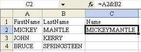
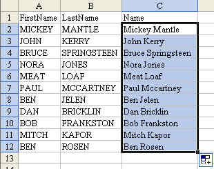
This is a good start. However, we really should concatenate first name, a space, and last name. Try this formula:
=A2&" "&B2
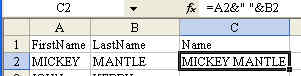
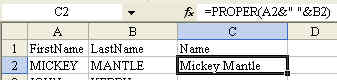
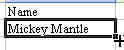
Then, the question is: do you want to scream MICKEY MANTLE, or would you rather say Mickey Mantle? If you want to change the name to proper case, use the =PROPER() function.
=PROPER(A2&" "&B2) [Note: see my comment to this message.]
Next, you want to copy the formula down to all of the cells in the column. A shortcut method for doing this is to double-click the fill handle while cell C2 is selected. The fill handle is the darker square dot in the lower right corner of the cell pointer. The dot looks like this:
 When your mouse pointer is near the dot, the mouse pointer changes to a cross like this. When your mouse pointer is near the dot, the mouse pointer changes to a cross like this.
Double click and the formula will be copied down to all of the cells in the range.
Note: Excel uses the column to the left when figuring out how far to copy cells after the double click. If you happened to have a blank cell in B8, this trick would stop at row 7. Leave cialis tadalafil 5mg it to Cher to cause a problem.
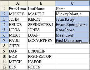
If this is the case, you might want to grab the fill handle and drag down to all of the rows in order to copy the formula. Note 2: The Proper function is excellent, but it does not properly capitalize last names like McCartney (See cell C7). You will have to manually go through and capitalize the C after the Mc. It would also have a problem with VanHalen. Is this a pain? Yes – but it is easier to fix a few cells than to retype everything in proper case.
Converting Formulas to Values Now that you have Firstname Lastname in column C, you might be tempted to delete columns A & B. You can't do this yet. If you would delete columns A & B, all of the formulas in column C would change to the #REF! error. This error is saying, "Hey – you told me the value in this column should be from A2 & B2, but you deleted those cells so I don't know what to put here!".
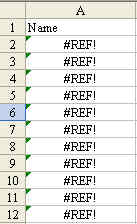
The solution is to change the formulas to values before you delete columns A & B. Follow these steps:
-
Highlight the range of cells in column C
-
Copy those cells to the clipboard using your favorite method (The 4 methods to choose from: Ctrl+c, or Edit – Copy from the menu, or the clipboard icon on the toolbar, or right-click and choose copy).
-
Without unselecting the cells, from the menu, choose Edit > Paste Special. From the Paste Special dialog box, choose Values and then OK. This step will paste the current value of each cell in the range back into the cell. Rather than having a formula, you will now have a static value. It is safe to delete columns A & B.
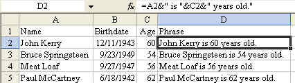
Joining a cell containing text to a cell containing a number In general, this will work out fairly well. In the image below, I've used the formula to build a phrase containing a name in column A with an age in column C.
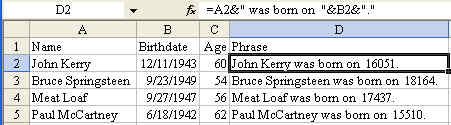
The trick is when the number is displayed in one format and you want it to be used in another format. Dates are a classic example of this. The date of December 11 1943 is actually stored as a number of days since January 1 1900. If I try to join the text in column A with the date in column B, I get a silly looking result
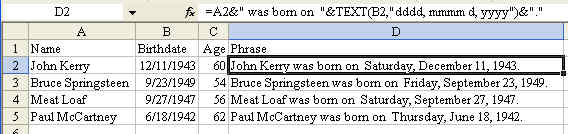
The solution is to use the =TEXT() function. The text function requires two arguments. The first argument is a cell containing a number. The second argument is a custom number format that indicates how the number is to be displayed. The following formula will produce a nicely formatted result.
There are a lot of cool techniques that were covered in this tip.
-
A formula to join 2 columns of text using the ampersand as a concatenation operator
-
How to join a cell to a text value
-
How to use the PROPER function to change names to proper case
-
Why you get a #REF! error
-
How to use Paste Special Values to convert formulas to values.
-
Joining a cell containing text to a cell containing a number
-
Using the TEXT function to control the display of a date in a formula.
This tip was originally published on September 12, 2004. The permanent URL for this page is http://www.mrexcel.com/tip074.shtml.
|